University at Buffalo (UB)


Physics Asks Big Questions
The Department of Physics offers vigorous, cutting-edge interdisciplinary research programs in new materials, nanoscience, quantum devices, biomolecular physics, complex systems, cosmology, high-energy physics and atmospheric physics. For recent news and activities please see our newsletter Interactions.
The Department is committed in providing a fair, just, safe, supportive, and equitable place for all to learn about physics and to perform ground-breaking research. Please read the Department's full statement on Diversity, Equity, and Inclusion here.
Prospective Students


Meet Our Faculty
Department Highlights
Announcements
Openings for Faculty Position
Follow the links at UB Jobs: Faculty (Assistant, Associate, or Full Professor), Physics and Associate or Full Professor, Physics
Summer & Winter Online Physics Courses
The Department of Physics offers five online "Intro to Physics" classes during the summer and winter breaks.
Information for Force Registration
If you require Force Registration, Registration for Independent Study, or Registration for Graduate Research, please see Information for Current Students.